 Oko Dot All In One Technology Solutions By Likhon Hussain
Excel is full of hidden tools that can completely transform your work, but most people will never discover them. Today, I’m revealing in this article five hidden tools to improve productivity and simplify your life.
By the end of this article, you’ll be wondering how you ever managed without them. My favorite Excel tool is number four. Let me know in the comments which are your favorite at the end of this article.
Tool No 01 : Quick Analysis Tool
Okay, let’s dive in and unlock these secret tools. If you’ve ever received a new dataset and not been sure where to start, in the Quick Analysis tool you have a load of shortcuts to help you make sense of it at your fingertips.
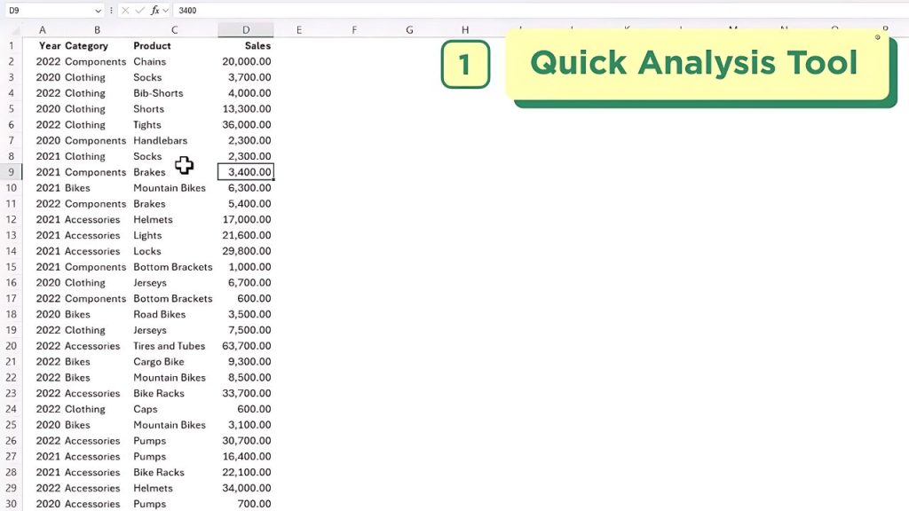
Here I’ve got a table of sales by year, category, and product, and I can simply press Ctrl + Q, and up pops a load of tools I can access with one click. For example, under charts, I can quickly see my sales by category.
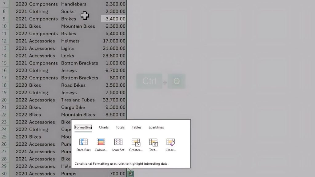
I’ll click on it and it inserts a new sheet including a pivot table and chart. From here, I can continue to work with the pivot table and chart to further customize them to my liking. Here I have some data on the daily intake of fruit and vegetables, and this sea of numbers is a bit difficult to make sense of.
Let’s see what Quick Analysis can do. I’ll start by selecting the numbers, Ctrl + Q, and under Formatting, we’ve got data bars, color scales, and icon sets. Hovering over them, I get a preview of how it’s going to look.
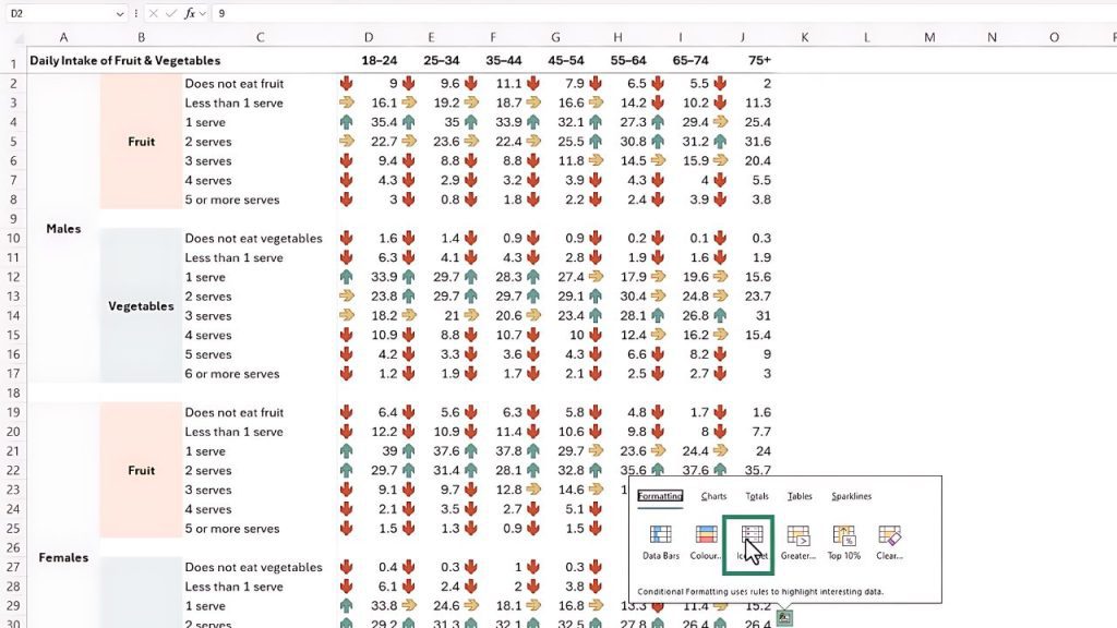
The data bars look pretty good. With one click, I’ve now got data bars to help me interpret my data. It would also be useful to know what the average is. I can do that with Ctrl + Q, and then under Totals, scroll across and choose Average.
This inserts a new column for me, and all I need to do is delete a few cells that have the #DIV! errors and give it a heading. I’ll insert another column because another cool feature is sparklines. Ctrl + Q on the Sparklines tab. I think the columns will be best. Let’s add those. Let’s give them a different color.
Now I can easily see at a glance that the younger generations are not big fruit and vegetable consumers compared to older generations, which was really difficult to see without these tools to help visualize the data. Now, if I select the data again and Ctrl + Q, you’ll notice there are loads more tools available and you can try these for homework.
Tool No 02 : Excel Flash Fill
This next tool can clean all kinds of messy data with a keyboard shortcut. Here I’ve got a list of names and I want to separate them into first name and last name. So I’ll just enter an example for the first row and then Ctrl + E for Flash Fill, and it extracts all the first names.
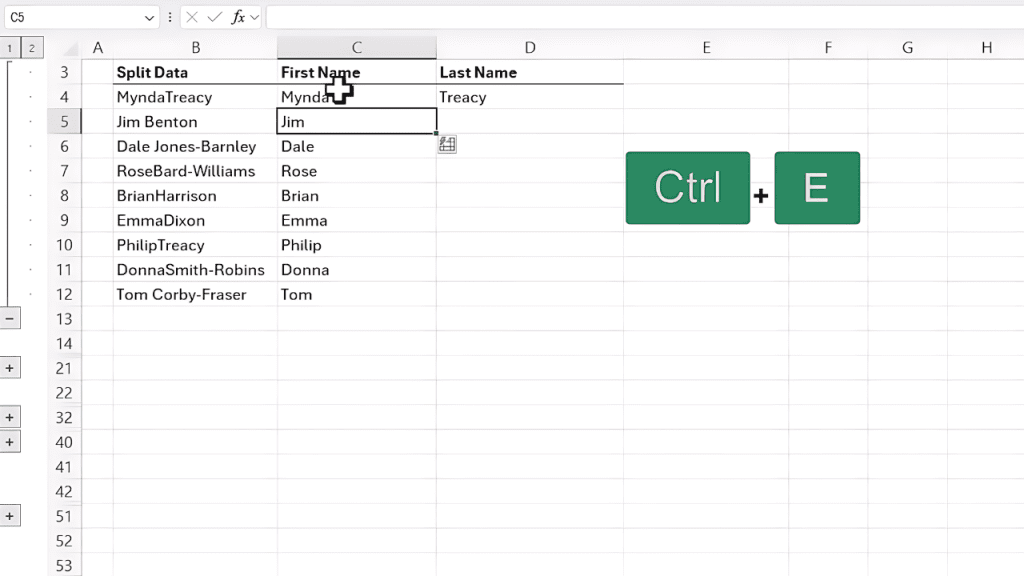
Let’s repeat for the last names, Ctrl + E, and it’s inserted the last names, but it’s got a couple wrong. So we can see here this should be a Jones-Barnley. By just correcting one of them, it now knows how to treat the rest.
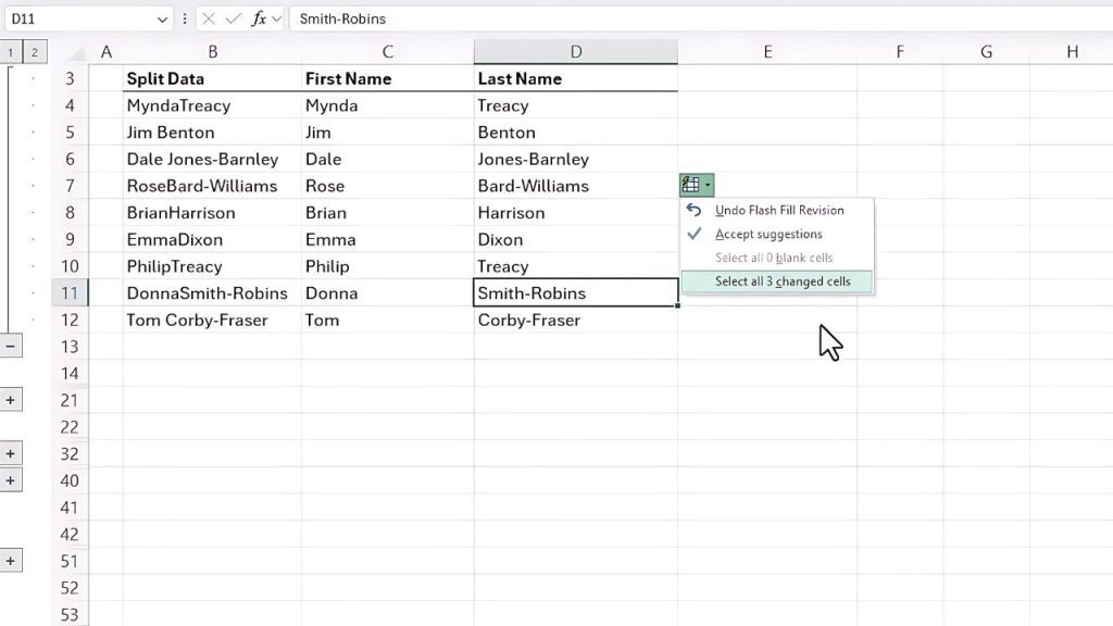
Now notice the Flash Fill menu appears and I can click on the drop-down to undo the revision, accept the suggestions, or select all three changed cells. Or I can just continue on, and it will assume I’ve accepted the suggestions.
Now there are tons of patterns you can have Flash Fill work with. For example, here I can have it construct an email address from the first and last names, then Ctrl + E, and it completes the rest for me. Now there are loads of other ways that you can use Flash Fill, and I’ve got some different examples here in the file that you can try for homework.
Tool No 03 : Drag to Fill
This might sound crazy, but you should stop using copy and paste because this can be more time-consuming than what I’m about to share with you. Here I have some formulas that calculate the sales, the cost of goods sold, and the profit.
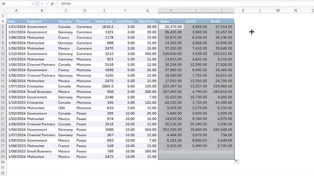
I want to copy these formulas down, so I can double-click the bottom right corner and it fills down. But noticed it messed up my formatting. So let’s Ctrl + Z to undo that. Another way I could copy it down is to copy it and then paste special, formulas.
That does the job, but it’s a load of clicks. So let’s Ctrl + Z to undo that. Instead of copying and pasting, I can right-click the fill handle and drag it down. When I release, I get a menu that allows me to choose Fill Without Formatting.
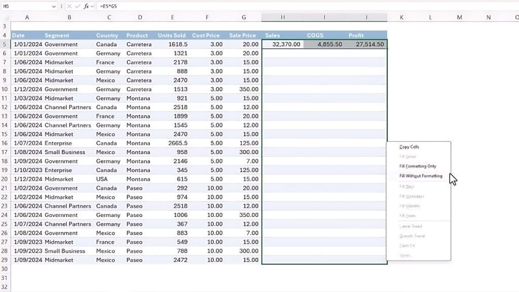
Now if we look in the cells, you can see it’s copied down my formulas, and my formatting isn’t messed up. At first, it’ll feel weird right-clicking and dragging, but you get used to it after a while.
Tool No 04 : Excel Custom Filter
This next shortcut is my favorite. It’s great for working with large data sets, enabling you to cut through the noise and find exactly what you need. For example, let’s say I wanted to focus on data for France. I can press the menu key. This brings up the right-click menu.
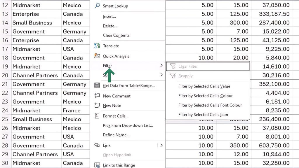
Here I want to filter. So you can see ‘e’ in Filter is underlined. So I need to press E. Then I want to filter by the selected cell’s value. So that’s V. Now my table is filtered for France. I have filter buttons for every column. Now I can continue applying filters.
For example, let’s say I want to only see data for the government. So again, the menu key, E, V. And maybe I only want to see the Montana product. So menu key, E, V, and you’ll get quicker and quicker at it the more you use it.
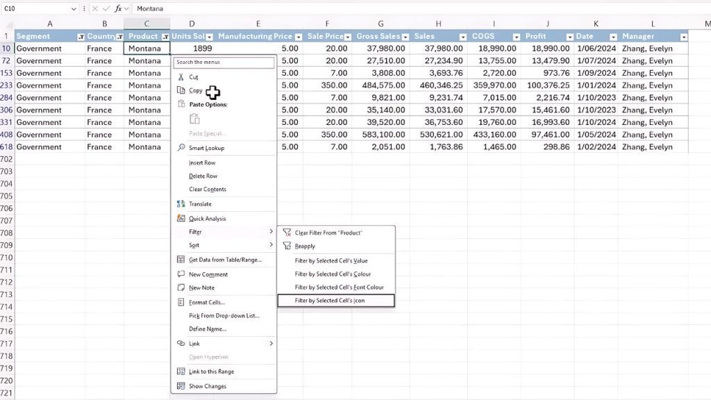
Now I have much less data to focus on, making it easier to find what I need. And of course, I can use the filter buttons to apply further filtering. Or I can click the menu key and access the other filter options here.
If you want to clear filters, you can do it one by one via this menu. Or you can go to the Data tab of the ribbon and click the Clear Filter button. Now for homework, check out the other shortcuts in the menu key. For example, ‘O’ for Sort.
Tool No 05 : Navigation Pane
Navigating through a workbook with countless sheets, tables, and charts can be like looking for a needle in a haystack. With the Navigation pane, we can get an instant overview of our workbook so we can quickly and easily find and access different elements.
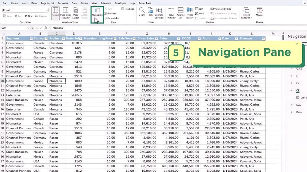
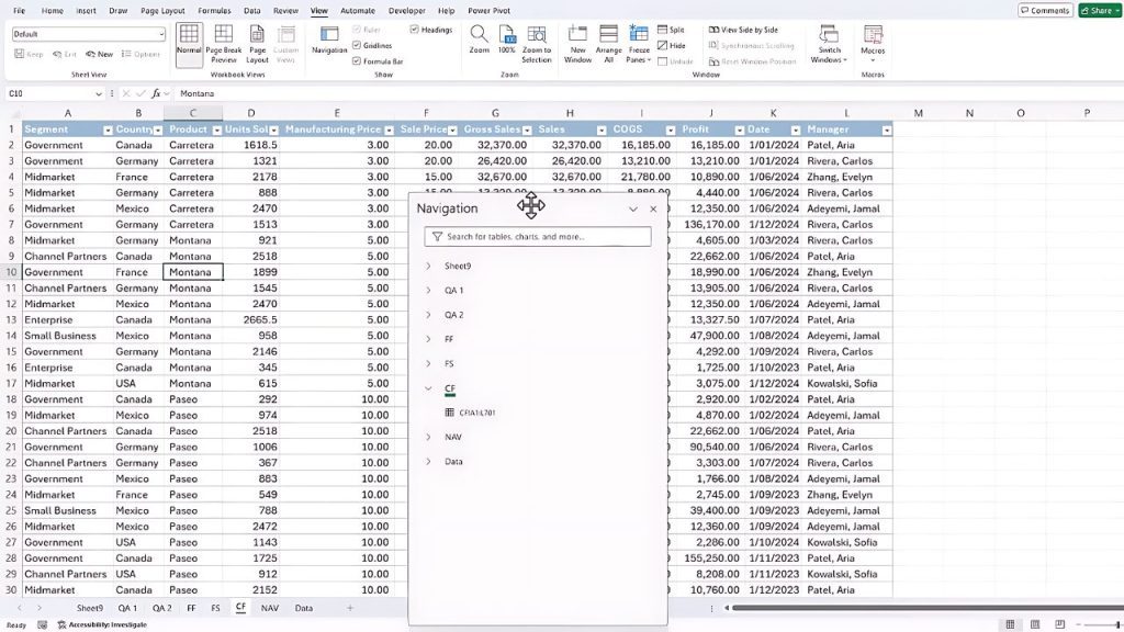
To access the Navigation pane, go to the View tab and then click on Navigation. This opens the pane on the right-hand side. You can unlock it by left-clicking and dragging. Now it’s mobile. Alternatively, you can dock it to the left-hand side if you prefer.
Clicking on one of the sheets takes you to that sheet and exposes the elements available there. You can select the elements from the Navigation pane, and you can see the chart is now selected in the worksheet.
If I expose one of the other sheets, you’ll notice it also makes ranges that contain data available. So I can click on this, and it takes me to that sheet. It also selects the table of data. Now the search bar at the top of the Navigation pane allows you to type and filter for specific tables or charts, for example.

You can see how I’ve got all the charts available. It also shows me the chart titles so I can easily select the correct chart. This is especially useful in large workbooks with numerous items. By default, all charts start with the name Chart, so they’re easy to find.
But this also applies to pivot tables, tables, shapes, and other objects, so you can search for them by their default name. Or you can name elements in line with how you want to search for them. For example, let’s say I want to rename these charts based on the intake of fruit and vegetables. Instead of calling it Chart 1, I can right-click and rename it.
The options you have in the right-click menu here will differ depending on the type of element. So I can rename this Intake 1 and click OK, then repeat for each chart. Now I can simply type in Intake to filter my list of elements based on that name. You can see I have charts and ranges named accordingly.
So I’ve got all of my objects and elements in one succinct list, making it super quick and easy to jump to them. If I want to navigate to a range, I can click on it, and it selects it. All this is the range of cells that I’ve named in the name box up here, so they’re super quick and easy to jump to from the Navigation pane.
Read More : Top 7 Fastest Growing Instagram Niches to Make Money in 2024